How To Make A Calibration Curve: A Guide (2024)

Calibration curves are essential for accurate chemical analysis. Many lab technicians struggle to create precise calibration curves, which can lead to errors in measurements and compromised data integrity. This frustration is common, yet avoidable with the right guidance.

This article provides a clear, step-by-step guide on how to make a calibration curve effectively. We cover the basics, common pitfalls, and tips for improving accuracy.

By the end of this guide, you will have the knowledge to produce reliable calibration curves, ensuring your chemical analyses are both accurate and dependable.

What is a calibration curve?

A calibration curve is a graph used in chemistry to find the amount of a substance in an unknown sample. We make the curve by testing known amounts of the substance, called standards.

We measure the instrument's response to each standard, like voltage or light absorption. Then we plot these measurements on a graph against the known amounts of the substance.

The resulting line shows the relationship between the instrument's response and the actual amount of the substance. By measuring an unknown sample and finding its response on the curve, we can determine its unknown amount. Calibration curves are essential for accurate chemical analysis using instruments.

Now that you know what a calibration curve is, let’s look at its applications in various chemical analyses.

Applications Of Calibration Curves In Various Chemical Analyses

Calibration curves are used in many chemical analyses. They are crucial in methods like spectroscopy and chromatography. These curves help in measuring the concentration of different chemicals accurately:

1) Spectroscopy (UV-Vis, AAS, etc.)

Ultraviolet-Visible Spectroscopy (UV-Vis): In UV-Vis, molecules absorb light at specific wavelengths. A calibration curve is made by measuring the absorbance (amount of light absorbed) of standard solutions at a chosen wavelength. The curve relates absorbance to the concentration of the analyte. By measuring the absorbance of an unknown sample at the same wavelength and using the curve, we can determine its concentration.

Atomic Absorption Spectroscopy (AAS): AAS works by atomizing a sample and measuring the light absorbed by these atoms at specific wavelengths. Similar to UV-Vis, standards with known concentrations are used. The instrument measures the amount of light absorbed by each standard solution. Plotting this against the known concentration creates a calibration curve. By measuring the light absorbed by an unknown sample and using the curve, we can determine its concentration.

2) Chromatography (HPLC, GC, etc.)

High-Performance Liquid Chromatography (HPLC): HPLC separates components in a mixture based on their interaction with a stationary phase. Calibration curves are crucial for quantifying specific components. Standard solutions containing known amounts of the analyte are injected, and their retention times (time taken to pass through the column) are recorded. A plot of the peak area (detector response) versus the concentration of the analyte in each standard creates the calibration curve. By injecting an unknown sample and measuring its peak area at the same retention time, we can determine its concentration using the curve.

Gas Chromatography (GC): Similar to HPLC, GC separates components based on their volatility. Standard solutions with known concentrations of the analyte are injected, and their retention times are recorded. A plot of peak area versus concentration of the analyte creates the calibration curve. By injecting an unknown sample and measuring its peak area at the same retention time, we can determine its concentration using the curve.

3) Immunoassays

Immunoassays rely on the specific interaction between antibodies and antigens. Calibration curves are used to quantify the amount of an analyte (antigen) in a sample. Standard solutions containing known amounts of the analyte are used. These standards compete with a labeled antigen for binding to a specific antibody. The amount of labeled antigen bound is measured and plotted against the known concentration of the analyte in each standard, creating the calibration curve. By measuring the labeled antigen bound in the presence of an unknown sample and using the curve, we can determine the unknown analyte concentration.

4) Environmental Analysis

Calibration curves play a vital role in environmental analysis, where monitoring pollutant levels is crucial. Standard solutions with known concentrations of pollutants like metals, pesticides, or organic compounds are prepared. These standards are analyzed using various techniques like spectroscopy, chromatography, or mass spectrometry. The instrument's response for each standard is plotted against its known concentration, creating the calibration curve. By analyzing environmental samples (water, soil, air) using the same technique and measuring the instrument's response, we can determine the concentration of the pollutant in the sample using the calibration curve.

Calibration curves in chemical analysis provide a basis for understanding their significance. We will explore their practical applications in various fields, along with their advantages and disadvantages. Understanding calibration curves' fundamentals and applications helps ensure accurate chemical analysis.

Advantages and Disadvantages of Calibration Curve

Calibration curves are easy to use. They are also accurate. But, they can be wrong if we don't make them carefully. Let’s have a look at the pros and cons of Calibration Curve:

Advantages of Calibration Curve

1) Accuracy: Calibration curves allow for accurate quantification of analytes in a sample by comparing the signal intensity of the unknown sample to the known standards.

2) Sensitivity: Calibration curves can be used to determine the sensitivity of an analytical method, which is the ability to detect and measure small changes in the concentration of an analyte.

3) Linearity: Calibration curves provide a linear relationship between the signal intensity and the concentration of the analyte, which simplifies data analysis and interpolation.

Disadvantages of Calibration Curve

1) Sample Matrix Effects: The presence of other components in the sample matrix can interfere with the signal intensity of the analyte, leading to inaccurate quantification.

2) Standard Preparation: Preparing accurate and reliable standards is crucial for constructing a calibration curve, which can be time-consuming and requires expertise.

3) Limited Range: Calibration curves are typically linear over a specific concentration range, and extrapolation beyond this range may lead to unreliable results.

To use calibration curves effectively, it’s important to understand the fundamentals behind them.

Understanding the Fundamentals of Calibration Curve

Analytical chemistry relies heavily on the relationship between the signal produced by an instrument and the concentration of the analyte (the component being measured) in a sample. This understanding is crucial for accurate and reliable analysis.

Relationship between instrument signal and analyte concentration

In analytical chemistry, various instruments generate a signal in response to the presence of an analyte. This signal can take many forms, such as voltage in an electrochemical sensor, light absorption in a spectrophotometer, or mass-to-charge ratio in a mass spectrometer. The key principle is that the strength or intensity of this signal is directly proportional to the concentration of the analyte in the sample.

For example, imagine measuring lead concentration in water using an atomic absorption spectrometer (AAS). As the concentration of lead in the sample increases, the AAS absorbs more light at a specific wavelength. This translates to a stronger signal on the instrument, indicating a higher lead concentration.

Linear relationship and deviations

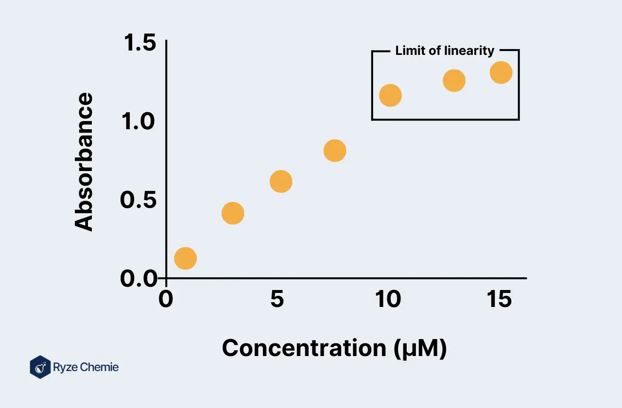
Ideally, the relationship between instrument signal and analyte concentration is linear. This means that a graph plotting these two values will yield a straight line. In this linear range, small changes in concentration result in predictable changes in the signal. This makes it easy to calculate the concentration of an unknown sample by measuring its signal and referring to the calibration curve (a graph generated using standards with known concentrations).

However, deviations from linearity can occur. At very low or very high concentrations, the relationship may become non-linear. This can happen due to various factors, such as saturation of the instrument's detector or limitations of the chemical reactions involved in the analysis. It is crucial to identify and operate within the instrument's linear range for accurate results.

Non-linear relationship

In some cases, the relationship between instrument signal and analyte concentration may not be linear over the entire concentration range. This is known as a non-linear relationship. Non-linearity can manifest in different forms, such as a curve that deviates from linearity at high or low concentrations or a sigmoidal curve.

Several factors can contribute to non-linearity, including:

Saturation: At high analyte concentrations, the instrument's detector may become saturated, leading to a decrease in sensitivity. This can result in a non-linear response, where the signal does not increase proportionally with increasing concentration.
Chemical Equilibrium: In some systems, chemical reactions or equilibria can affect the relationship between signal and concentration. For example, in acid-base titrations, the pH of the solution can influence the ionization of the analyte, leading to a non-linear titration curve.
Matrix Effects: The presence of other components in the sample matrix can interfere with the analyte's signal, causing deviations from linearity. Matrix effects can be complex and challenging to account for accurately.

Addressing Non-Linearity

When encountering non-linearity, several strategies can be employed to address the issue:

Linearization Techniques: In some cases, it may be possible to transform the non-linear data into a linear form using mathematical transformations, such as logarithmic or power transformations. This can facilitate the use of linear regression for calibration.
Segmentation: The calibration curve can be divided into multiple linear segments, each with its own linear equation. This piecewise linear approach can provide a better fit for non-linear data.
Non-Linear Regression: Non-linear regression techniques can be used to fit a non-linear model to the data. This approach allows for a more accurate representation of the true relationship between signal and concentration.

It is important to note that non-linearity can introduce complexities and uncertainties into quantitative analysis. Careful consideration and appropriate mathematical treatment are necessary to ensure reliable results when working with non-linear calibration curves.

Importance of choosing the right analytical technique

The choice of analytical technique significantly impacts the relationship between instrument signal and analyte concentration. Different techniques have varying sensitivities and linear ranges. Selecting the right technique ensures you can measure the analyte within its linear range and achieve the desired level of accuracy and detection limits.

For instance, measuring trace levels of mercury in water might require a highly sensitive technique like inductively coupled plasma mass spectrometry (ICP-MS) due to its low concentration. Conversely, measuring the concentration of salt (sodium chloride) in seawater might be well-suited for a technique like conductivity measurement, which has a wider linear range for high salt concentrations.

Selection of standards:

Standards are the foundation of accurate quantitative analysis. They are solutions or materials with known concentrations of the analyte used to calibrate the instrument and construct the calibration curve. Choosing the right standards is essential for reliable results.

Choosing the appropriate standard material

The standard material should be as similar to your samples as possible in terms of matrix composition (the surrounding components). This helps minimize any matrix effects that could interfere with the instrument's response. For example, if analyzing lead in blood, using a lead standard prepared in blood would be ideal. However, if blood is unavailable, using a lead standard prepared in a similar biological matrix like serum might be acceptable.

Reference standards vs. working standards

There are two main types of standards used in analytical chemistry:

Reference standards: These are highly pure materials with certified concentrations traceable to national or international standards organizations. They are used to prepare working standards and ensure the accuracy of the entire measurement process. However, due to their cost and limited availability, reference standards are not used for routine analysis.
Working standards: These are prepared by diluting reference standards or commercially available standard solutions to concentrations closer to the expected range of the analytes in your samples. Working standards are used for daily calibration and construction of the calibration curve. It is recommended that fresh working standards are prepared regularly to minimize any degradation or contamination effects..

By understanding the relationship between instrument signal and analyte concentration, the importance of linearity, and the selection of appropriate analytical techniques and standards, you can ensure the accuracy and reliability of your chemical analyses. This foundation is essential for generating meaningful data and drawing sound conclusions from your experiments.

With these fundamentals in mind, let’s move on to the step-by-step process of making a calibration curve.

How To Make A Calibration Curve

Creating a calibration curve is essential in quantitative analysis to determine the concentration of an analyte in a sample. This step-by-step guide will help you understand how to make a calibration curve effectively:

Preparing for Calibration Curve Construction

Step 1: Planning and Preparation

Define the Analyte of Interest

Identify the specific analyte you need to measure. Knowing the analyte will guide you in selecting the appropriate analytical method.

Select the Analytical Method Based on Sensitivity and Selectivity

Choose an analytical method that is sensitive and selective for the analyte. This ensures accurate detection and quantification.

Choose the Concentration Range for the Calibration Curve

Decide on a concentration range that encompasses the expected concentrations in your samples. This range should provide a clear, linear relationship between concentration and instrument response.

Determine the Number of Standards to be Prepared

Prepare at least five standards. More standards can provide a more reliable calibration curve. The standards should cover the entire concentration range.

Step 2: Making the Stock Solution

Calculations for Preparing a Concentrated Stock Solution

Calculate the amount of analyte needed to prepare a concentrated stock solution. Use accurate measurements to ensure the solution's concentration is correct.

Importance of Accurate Weighing and Dilution Techniques

Accurate weighing is crucial to preparing a reliable stock solution. Use precise dilution techniques to ensure consistency and accuracy when making subsequent dilutions.

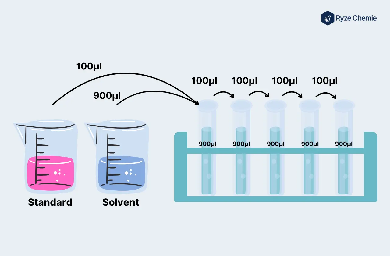
Step 3: Serial Dilutions for Calibration Standards

Description of the Serial Dilution Process

Serial dilution involves systematically diluting the stock solution to achieve a series of standards with known concentrations. Each dilution should reduce the concentration by a consistent factor.

Calculations for Preparing Dilutions

Calculate the volumes required for each dilution. A dilution table can simplify this process, ensuring accuracy.

Best Practices for Pipetting Techniques to Minimize Errors

Use proper pipetting techniques to avoid errors. This includes pre-wetting the pipette tip, dispensing at a consistent angle, and avoiding air bubbles.

Running the Calibration and Acquiring Data

Step 4: Sample Preparation and Measurement

Sample Matrix Considerations and Potential Interferences

Consider the sample matrix and identify any potential interferences that could affect the measurement. Choose preparation methods that minimize these interferences.

Following Standardized Protocols for Sample Preparation

Adhere to standardized protocols for preparing your samples. Consistency in preparation ensures reliable results.

Operating the Analytical Instrument According to Manufacturer's Instructions

Follow the manufacturer’s instructions for operating the analytical instrument. This ensures the instrument functions correctly and provides accurate readings.

Recording Instrument Response (Signal) for Each Standard and Replicate Measurements

Measure and record the instrument response for each standard. Perform replicate measurements to ensure reliability and account for any variability.

Data Analysis and Interpretation

Step 5: Plotting the Calibration Curve

Choosing the Appropriate Axes (Concentration on X, Signal on Y)

Plot concentration on the x-axis and the corresponding signal on the y-axis. This standard approach helps visualize the relationship between the two variables.

Plotting the Data Points and Including Error Bars

Plot the data points on a graph. Include error bars to represent the standard deviation, showing the variability in your measurements.

Step 6: Linear Regression Analysis

Importance of a Linear Relationship for Accurate Quantification

A linear relationship between concentration and signal is crucial for accurate quantification. It ensures that the calibration curve can reliably predict unknown concentrations.

Performing Linear Regression to Obtain the Best-Fit Equation (y = mx + b)

Use linear regression to determine the best-fit equation for your data. The equation should be in the form y = mx + b, where y is the signal, m is the slope, x is the concentration, and b is the intercept.

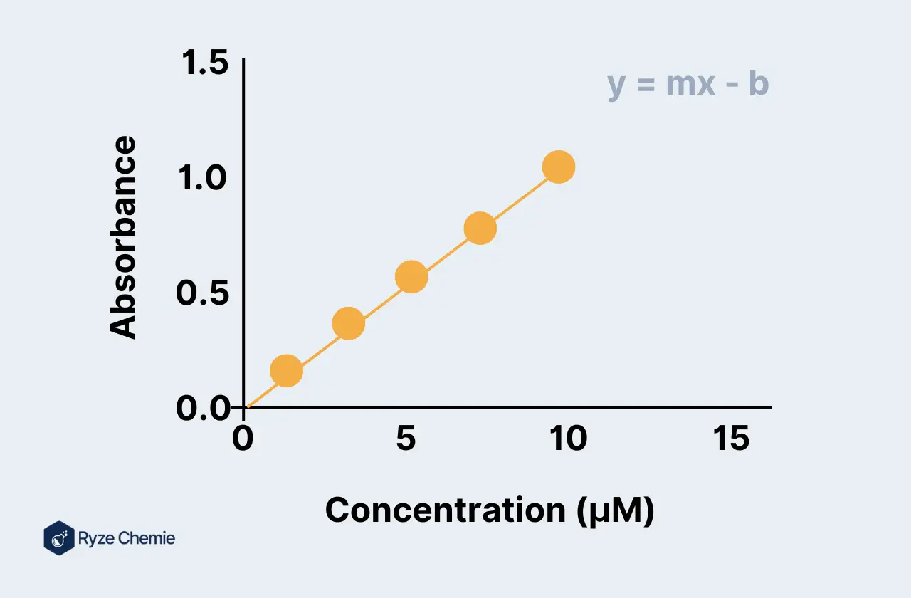
Evaluating the R-Squared Value

Assess the R-squared value of the regression. This value indicates the goodness of fit; an R-squared value close to 1 suggests a strong linear relationship.

Step 7: Examining Deviations from Linearity

Identifying Outliers and Potential Reasons for Non-Linearity

Look for outliers or deviations from the linear trend. Identify possible reasons for non-linearity, such as instrumental errors or sample contamination.

Excluding Outliers if Justified and Repeating Measurements

Exclude outliers if there is a justified reason. Repeat the measurements to ensure accuracy and reliability.

Using the Calibration Curve for Unknown Samples

Step 8: Measuring Unknown Samples

Preparing and Analyzing Unknown Samples Using the Same Protocol

Prepare the unknown samples using the same protocols as the standards. Consistency is key to obtaining reliable results.

Recording Instrument Response for Unknown Samples

Measure and record the instrument response for each unknown sample. Ensure the measurements are within the calibration range.

Step 9: Calculating Unknown Concentration

Using the Calibration Equation (y = mx + b) to Determine Unknown Concentration

Use the calibration equation obtained from linear regression to calculate the unknown concentration. Substitute the measured signal into the equation to find the concentration.

By following these steps, you can create an accurate calibration curve and use it to determine the concentration of unknown samples. Accurate calibration curves are essential for reliable quantitative analysis in chemical laboratories.

Once you know the steps, it’s important to follow best practices and consider various factors to ensure accuracy.

Best Practices and Considerations to Consider While Making the Calibration Curve

It’s crucial to follow certain best practices when making calibration curves to achieve the most reliable results. This part of the article outlines these key considerations:

1) Importance of using replicates and calculating standard deviation

Replicate measurements are essential for assessing the reproducibility of your calibration curve. Prepare and analyze multiple replicates (at least 2-3) of each concentration level in your curve. This allows you to calculate the standard deviation (SD), which reflects the spread of data points around the average value. A low SD indicates good precision and reduces uncertainty in your measurements.

How it helps: Including replicates helps identify outliers or errors in a single measurement. The SD provides a quantitative measure of the variability in your data, allowing you to judge the reliability of the calibration curve.

Example: You prepare three replicates of a 10 ppm standard solution and measure their instrument response. The response values are 12.5, 12.2, and 12.8. The calculated SD is 0.3 ppm. This small SD suggests good precision in your measurements, strengthening the confidence in your calibration curve.

2) Quality control procedures: blank measurements, spike recoveries

Blank measurements assess background signals or contamination in your measurement system. Analyze a blank sample containing all reagents except the analyte. A high blank signal indicates potential contamination, which can affect your calibration curve and subsequent analysis.

Spike recoveries evaluate the efficiency of your sample preparation process. Add a known amount of the analyte (spike) to a sample matrix and analyze it alongside your calibration curve. Compare the measured concentration of the spiked analyte with the expected amount. Low recoveries suggest analyte loss during preparation, requiring corrective measures or adjustments to your calibration curve.

How it helps: Blank measurements help identify and address potential interferences, leading to more accurate calibration curves. Spike recoveries assess potential analyte loss during sample preparation, ensuring the validity of your analytical results.

Example: You analyze a blank sample, and the instrument response is negligible. This indicates a minimal background signal, which is suitable for proceeding with calibration. You spike a sample matrix with 10 ppm of the analyte and measure a concentration of 8.5 ppm after analysis. The recovery is 85%, suggesting a slight loss during preparation. You may need to adjust your calibration curve or consider modifying your sample preparation.

3) Maintaining calibration curves: frequency of updates

The frequency of calibration curve updates depends on several factors. Consider the stability of the analyte in solution, the instrument performance, and the desired level of accuracy.

Unstable analytes that degrade over time require more frequent calibration updates.
Instrument drift can lead to changes in signal response, necessitating recalibration.
High-precision analyses may require stricter calibration update schedules.

How it helps: Regularly updated calibration curves ensure consistent and reliable measurements. Outdated curves can lead to inaccurate results and unreliable data.

Example: You are analyzing a sample containing a light-sensitive compound. You decide to recalibrate the instrument every 4 hours to account for potential analyte degradation.

4) Data recording and documentation practices

Meticulous record-keeping is essential for maintaining a traceable and auditable analytical process. Maintain a detailed record of all calibration curve preparation steps, including:

Date of preparation
Source and concentration of stock standards
Preparation calculations for each concentration level
Instrument identification and settings
Raw instrument response data for all standards and replicates
Calibration curve equation and correlation coefficient (R^2)
Any observations or notes during the preparation or analysis

How it helps: Clear documentation allows for easy review, troubleshooting, and ensures data integrity. Proper records are crucial for demonstrating adherence to quality control protocols and regulatory requirements.

Example: You create a logbook entry for your calibration curve. It includes the date, source of a 1000 ppm stock solution, calculations for preparing a 5-point calibration curve, instrument settings, response data for replicates of each standard, the generated calibration equation (y = mx + b) with R^2 = 0.998, and a note mentioning the use of new pipettes.

By following these best practices and considerations, you can create reliable calibration curves that form the foundation for accurate and trustworthy analytical results. Remember, consistent quality control procedures, meticulous documentation, and regular updates are crucial for maintaining the integrity of your calibration curves.

Conclusion

Creating a calibration curve is crucial for accurate chemical analysis. By following the steps outlined, you can ensure reliable and precise results.

Always prepare your standards carefully and measure them accurately. Plot the data points and draw the best fit line to create the curve. Regularly check and maintain your equipment to ensure consistent performance.

Calibration curves help you determine unknown concentrations effectively. With practice, you will become more proficient in this essential technique. Use this guide as a reference to enhance your skills and confidence in creating accurate calibration curves.